Module 4 — RAG: Retrieval Augmented Generation¶

In this module

Understand why RAG exists — hallucination, knowledge cutoff, and private-data blindness are the three problems it solves simultaneously.
Trace the full RAG pipeline from raw document to generated answer: chunk → embed → store → retrieve → augment → generate.
Learn the chunking and embedding decisions that most affect retrieval quality.
Know when to reach for a vector database versus when to just stuff everything in the context window.
Distinguish naive RAG from advanced RAG (re-ranking, hybrid search) and know when the upgrade is worth it.

Time: ~50 min · Lab: Lab 4 — Vanilla RAG

Why this matters¶

Every LLM ships with a fixed body of knowledge frozen at training time, with no awareness of your private data and a tendency to invent plausible-sounding answers when it doesn't know something. For a chatbot answering questions about last quarter's support tickets or your internal API docs, those three problems — hallucination, knowledge cutoff, and private-data blindness — combine into a single show-stopper. RAG is the standard engineering fix: pull the right documents at request time and hand them to the model as context, so the model is answering from your data, not its memory.

The core problem RAG solves¶

LLMs have three structural limitations that no amount of prompting alone can fix:

Hallucination. Next-token prediction produces the most probable continuation, not a verified fact. Ask a model about an event it wasn't trained on and it will confidently generate something — usually wrong. This is a feature of how the model works, not a bug to be patched away.

Knowledge cutoff. The model's weights encode the world up to a specific date. Anything after that — your latest release notes, last week's incident postmortem, regulatory updates — simply doesn't exist inside the model.

Private-data blindness. Models are trained on public data. Your internal wiki, your proprietary codebase, your customer contracts — the model has never seen them and cannot reason about them without being given the text.

RAG solves all three in one move: at query time, retrieve the relevant passages from your corpus and inject them into the prompt. The model now has the right context; it answers from that, not from memory.

RAG as a pipeline pattern¶

RAG is not a model; it is a pipeline pattern layered on top of a model. The software analogy is precise and useful: RAG is a database lookup before composing the API response. Your service doesn't hard-code every possible answer; it queries the right record at request time and composes the response from that data. RAG applies the same pattern to language generation: don't bake the knowledge into the model; look it up when you need it.

In plain words

RAG turns a closed-book exam into an open-book one. Instead of forcing the model to answer purely from memory (where it might misremember and "hallucinate"), you let it look up the relevant pages from your documents first and answer from what it just read. Same student, far better answers — because now it's quoting the book instead of guessing.

The whole pipeline at a glance — documents in, grounded answer out:

A RAG flow. Additional documents are (1) encoded by an embedding model and (2) indexed into a vector database. A user query is (3) encoded by the same embedding model and used to (4) run a similarity search against the vector database, which returns (5) similar documents. Those documents are combined with the query (6) to form the prompt sent to the LLM, which (7) produces the response.

The pipeline has two distinct phases — indexing (done offline, once per document corpus) and querying (done at request time, once per user query):

RAG pipeline — indexing offline, querying at request time:

flowchart TD
    subgraph INDEXING["INDEXING PHASE (offline)"]
        D["Raw documents"] --> C["Chunk<br/>(split into focused passages)"]
        C --> E["Embed<br/>(embedding model → vectors)"]
        E --> V["Vector DB<br/>(store vectors + text)"]
    end

    subgraph QUERYING["QUERYING PHASE (per request)"]
        Q["User question"] --> EQ["Embed query<br/>(same embedding model)"]
        EQ --> R["Retrieve top-k<br/>(cosine similarity search)"]
        R --> A["Augment prompt<br/>(inject retrieved chunks)"]
        A --> G["LLM"]
        G --> ANS["Grounded answer"]
    end

    V --> R

Each box is a separately replaceable component — swap the embedding model, the vector store, or the LLM without touching the others.

Chunking strategies¶

Chunking is the step that splits raw documents into the passages you will embed and retrieve. The size and method you choose directly determines retrieval quality — too large and retrieved chunks contain noise; too small and they lack enough context to be useful.

The two main strategies:

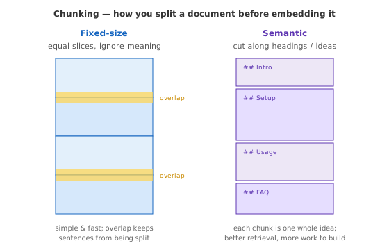
Fixed-size chunking. Split every N tokens with a small overlap (e.g. 512 tokens, 50-token overlap). Fast, predictable, and the right default for homogeneous text like support-ticket bodies or log entries. The overlap window prevents a sentence from being split exactly at the chunk boundary and losing its meaning.

Semantic chunking. Split on natural boundaries — paragraphs, headings, or sentences — and only then enforce a size limit. Better for structured documents like API reference pages or legal contracts where a heading-to-heading section is a coherent unit. More complex to implement but pays off when your documents have strong internal structure.

Two ways to cut the same document:

Two ways to chunk a document. On the left, fixed-size: the document is cut into equal-length slices, with a small highlighted overlap band shared between neighbouring slices so a sentence is not lost at the boundary. On the right, semantic: the document is cut along its headings, one chunk per section, so each chunk is a complete idea.

A useful mental model: chunking is like deciding how to split a codebase into individually reviewable pull requests. Too large and reviewers (the retriever) can't focus; too small and there's no context for each change. Aim for the smallest unit that is still self-contained.

Embeddings and why semantic search works¶

Embedding converts text into a dense vector — a list of numbers where similar meanings end up geometrically close together. The embedding step happens twice: once for every chunk during indexing, and once for the user's query at request time. The retriever then finds the stored chunk vectors nearest to the query vector.

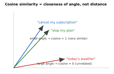
Semantic search / similarity search finds chunks by meaning, not keyword overlap: the question and every chunk are turned into embeddings (vectors), and retrieval returns the chunks whose vectors are "closest" to the question's vector. That is why "cancel my subscription" can match a chunk that says "end your plan" — no shared keywords required.

Cosine similarity is the usual measure of "closest." It compares the angle between two vectors, not their length: vectors pointing in nearly the same direction score near 1 (very similar), perpendicular vectors score near 0 (unrelated), and opposite directions score near −1. Using the angle rather than raw distance keeps the score about meaning and direction rather than how long or "loud" the text is — a short tweet and a long article on the same topic still score high if they point the same way.

Cosine similarity compares the angle between vectors: "cancel my subscription" and "stop my plan" sit at a small angle (high similarity), while "today's weather" is at a wide angle (unrelated).

In plain words

Think of every phrase as an arrow on a map. Cosine similarity asks "do these two arrows point the same way?" — not "how long are they?" Arrows pointing the same direction mean the same thing (score near 1); at right angles they're unrelated (near 0). That's why a short tweet and a long article on the same topic still match: same direction, different length.

The practical implication: if your users ask questions using vocabulary that differs from your documentation (end-user language vs. engineering language), semantic search handles that gap automatically. Keyword search — LIKE '%cancel%' — would miss it.

Vector databases¶

A vector database is a store purpose-built for one operation: given a query vector, return the top-k most similar stored vectors efficiently. Standard relational databases can store vectors but have no fast index for nearest-neighbour lookup; vector databases have this as their primary index.

Three you will encounter constantly:

Store	When to use
Chroma	Local development and prototyping; zero infrastructure; in-process or as a local server
Pinecone	Managed cloud service; handles scale and replication; simplest production path
pgvector	You already run Postgres; add the extension and keep your existing ops tooling

The API surface of all three is essentially the same: upsert(vectors), query(vector, top_k). The infrastructure decision is ops preference and scale, not a different programming model.

Naive vs advanced RAG¶

The pipeline described above is naive RAG: embed-index offline, cosine-retrieve at query time, stuff top-k chunks into the prompt. It works well for a large class of problems and is the right place to start.

Where it breaks down:

The top-k chunks by cosine score are not always the most relevant chunks — they are the most similar to the query vector, which is a proxy that sometimes fails on ambiguous queries.
Keyword-heavy queries ("error code 503 in checkout service") do not always find what semantic search finds; and semantic queries sometimes miss exact-match terms.

Advanced RAG addresses both:

Re-ranking adds a second pass after retrieval. The first-pass retriever returns a larger candidate set (top-20); a lightweight cross-encoder re-ranks them by relevance to the specific query and you keep only the top-5. Cross-encoders are slower but more accurate than cosine similarity because they see the query and the chunk together rather than separately. Cost: one extra model call per query.

Two-pass retrieval — cast a wide net cheaply, then sort precisely:

flowchart LR
  Q["Query"] --> R1["Retrieve top-20<br/>(fast cosine search)"]
  R1 --> RR["Re-rank by relevance<br/>(cross-encoder)"]
  RR --> K["Keep top-5"]
  K --> P["Augment prompt → LLM"]

The first pass is wide and cheap; the second pass is narrow and precise — like skimming twenty search results, then reading the five that actually answer your question.

Hybrid search fuses keyword search (BM25 or a full-text index) and semantic search, then combines their ranked lists (reciprocal rank fusion is the standard merge). You get the recall benefits of both: exact-match terms are caught by keyword search; paraphrases and synonyms are caught by semantic search. Cost: maintain two indexes.

Start with naive RAG. Add re-ranking when you observe the model citing wrong or tangentially relevant chunks. Add hybrid search when exact identifiers (product codes, error codes, version numbers) are in queries and semantic search misses them.

Agentic RAG goes one step further: instead of a single fixed retrieve-then-answer pass, an agent decides how to retrieve — rephrasing the query, retrieving in several rounds, and judging whether it has enough before answering. It cuts hallucination but introduces a new failure mode: stitching together two chunks that are actually about different things. The fix is citation grounding — require the model to attribute each claim to a specific chunk ID, so every statement is traceable back to its source. Reach for agentic RAG only once naive RAG's single pass is demonstrably not enough; it multiplies cost and latency.

When NOT to use RAG¶

RAG is the right tool when your corpus is too large to fit in the model's context window or changes frequently. But two situations make it unnecessary:

Small, stable data. If your reference material is 5,000 tokens of docs that change once a month, use context-window stuffing: put the whole thing in the system prompt. No vector database, no chunking, no retrieval pipeline to maintain. Simpler is better until the data grows past what the context window can hold.

Exact-match lookup. If the user is querying a structured record (order status, account balance, current inventory count), call your database directly via tool use and inject the result. RAG is for unstructured document retrieval; use the right tool for structured data.

A useful decision rule: if you would reach for a search engine rather than a database, RAG is likely the right fit. If you would reach for a SQL query, use function/tool calling to query the database and inject the result.

Choosing: prompt, long context, RAG, or fine-tuning?¶

There are four ways to get the right knowledge into a model's answer — from cheapest to heaviest:

Approach	What it is	Best when	Watch out for
Just prompt	put the facts directly in the prompt	the info is small, static, and you already have it	nothing to retrieve; doesn't scale to a big corpus
Long context	paste whole documents into a large window	a handful of docs, whole-document reasoning, rare change	usable quality often fades past ~25–50% of the stated window; slow and costly per call
RAG	retrieve the relevant chunks at query time	a large or changing corpus, many users, freshness matters	retrieval quality is the ceiling; you own a pipeline
Fine-tuning	further-train the weights on your data	you need a consistent style/format/behaviour	costly, needs data + ops; does not reliably add new facts

Two rules that hold up in practice:

Knowledge vs behaviour. Need the model to know new facts? → RAG (or context). Need it to behave a certain way consistently? → fine-tuning. Mixing these up is the most common mistake — fine-tuning to add facts is expensive and unreliable; RAG to change tone is awkward.
Long context doesn't kill RAG. Even with million-token windows, retrieval still wins for large or permissioned corpora, because usable context is often only a quarter to a half of the stated limit. The 2026 rule of thumb: use long context to reason over a focused evidence set, and use retrieval to choose what that set should be.

Start at the top of the table and move down only when you must — each step down adds cost and moving parts.

Mental model

RAG is the same pattern your API already uses when it hits a database before composing a response — except the "database" stores meaning vectors instead of rows, and the "compose" step is an LLM generating prose instead of JSON serialisation. The engineering discipline is identical: schema design (chunking), indexing (embedding), query optimisation (re-ranking), and cache vs. live-fetch tradeoffs (context stuffing vs. retrieval). You already know how to reason about these; RAG just moves them into the language layer.

Hands-on¶

Open Lab 4 — Vanilla RAG. You'll build the full pipeline by hand — chunk a small document set, embed it with OpenAI's text-embedding-3-small, store the vectors in Chroma, retrieve the most relevant chunks for a question, and generate a grounded answer — then watch the model correctly decline a question whose answer isn't in the documents.

Go deeper¶

Retrieval Augmented Generation (RAG) — Prompt Engineering Guide — The clearest written reference for RAG fundamentals; covers the pipeline, naive vs. advanced RAG variants, and practical implementation guidance in one page. Start here before going deeper.
RAG Explained — IBM Technology (YouTube) — A well-produced 8-minute visual explainer from IBM; animated diagrams walk through the indexing and querying phases side-by-side. Ideal if you learn faster from visuals than text.
What is Retrieval-Augmented Generation? — IBM Think — IBM's written reference article; strong on the business rationale and goes into RAG variants (corrective RAG, self-RAG) for when you hit the limits of vanilla RAG.
RAG: A Comprehensive Visual Walkthrough — Towards AI — Step-by-step visual walkthrough with diagrams at every stage of the pipeline; good for building the mental picture of how vectors and cosine similarity actually connect query to chunk.

Jargon recap¶

RAG · hallucination · knowledge cutoff · chunking · embedding · vector database · semantic search / similarity search · cosine similarity · retrieval · re-ranking · hybrid search · context window · long context · agentic RAG · citation grounding · fine-tuning

Check yourself¶

Try to answer before expanding — active recall is what makes it stick.

What three problems does RAG solve at once?

Hallucination (the model invents plausible answers), knowledge cutoff (it knows nothing after training), and private-data blindness (it never saw your internal docs). RAG fixes all three by retrieving relevant passages from your corpus at query time and injecting them into the prompt.

What are the two phases of a RAG pipeline?

Indexing, done offline once per corpus: chunk → embed → store in a vector DB. Querying, done per request: embed the query → retrieve top-k similar chunks → augment the prompt → generate a grounded answer. Each component is independently replaceable.

How do you choose between just prompting, long context, RAG, and fine-tuning?

Move down the list only as you must. Prompt when the facts are small and static; use long context for a handful of whole documents; use RAG for a large or changing corpus; fine-tune to change behaviour/style, not to add facts. Rule: RAG (or context) adds knowledge, fine-tuning changes behaviour.

When should you NOT use RAG?

When the data is small and stable (under a few thousand tokens that rarely change) — just stuff it in the system prompt. And for exact-match lookups of structured records (order status, balance) — query the database directly via tool use instead.

Key takeaways¶

RAG solves hallucination, knowledge cutoff, and private-data blindness in one pipeline by injecting retrieved context at request time rather than baking knowledge into model weights.
The pipeline is two phases: index offline (chunk → embed → store) and query at runtime (embed query → retrieve → augment → generate) — each step is independently replaceable.
Chunking and embedding quality drive retrieval quality; fixed-size with overlap is the right default, semantic chunking pays off for structured documents.
Start with naive RAG; add re-ranking when retrieved chunks are off-target, and hybrid search when exact identifiers appear in queries.
If your data fits in the context window and changes rarely, skip RAG — just put it in the system prompt.

Next: Agents →