Module 2 — How LLMs Are Built
In this module
- Understand how text becomes numbers through tokenization — and why token ≠ word.
- Grasp embeddings as a "semantic coordinate system" that lets math operate on meaning.
- Get the transformer architecture and attention in plain English — no equations.
- Know what pre-training actually trained the model on and what it "remembers."
- Distinguish fine-tuning from prompting at the level that matters to you: one changes the weights, one doesn't.
- Understand why RLHF is what makes a model feel helpful rather than just fluent.
- Know which runtime dials (context window, temperature, top-p) you'll turn in Lab 2.
Time: ~35 min · Lab: Lab 2 — First API Call
Why this matters
Every surprising or frustrating LLM behaviour — a model that counts tokens wrong, hallucinates a plausible-sounding lie, or gives a radically different answer when you nudge the temperature — traces back to a decision made during the build process. You don't need to build an LLM; you need a clear enough mental model of its internals that you can diagnose these behaviours, tune the dials deliberately, and explain to stakeholders why a 70B model is better for some tasks and a 7B model is better for others. This module builds that model.
Tokenization — text as numbers
Before a word of your prompt reaches the neural network, it goes through tokenization: the process of splitting your text into tokens and replacing each token with an integer ID from the model's vocabulary.
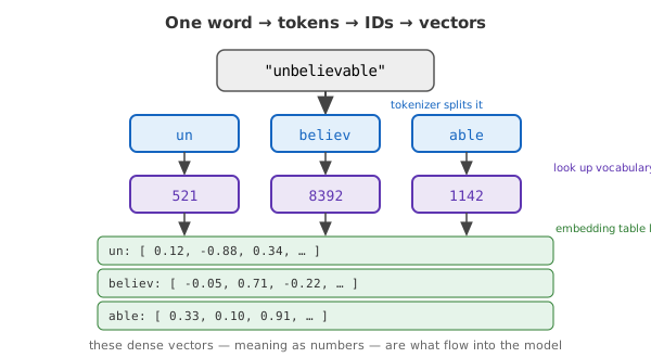
A token is roughly 3–4 characters of English text — not a whole word. The word
unbelievable might become three tokens: un, believ, able. The word I is a
single token. An emoji might be two tokens. This has practical consequences: a
"4,096-token context window" is about 3,000 words of English, but far fewer words
in Chinese or Finnish (which tokenize less efficiently with English-centric vocabularies).
The software analogy: think of tokenization as UTF-8 encoding, but at the word-fragment level. The model never sees raw characters; it only ever sees integer IDs into a vocabulary table. Every billing meter, every context limit, every "max_tokens" parameter in your API call is counting these IDs — not words, not characters.
Mental model
Tokens are the model's "bytes." Just as a C program operates on bytes regardless of what character encoding a human has in mind, an LLM operates on token IDs regardless of what words a human has in mind. Paste your prompt into Tiktokenizer and watch a single "word" become three tokens — the billing surprise becomes intuitive immediately.
How your text becomes a model output — the token pipeline:
flowchart LR
  Text["Text"] --> Tokenizer["Tokenizer"] --> IDs["Token IDs"] --> Transformer["Transformer"] --> Probs["Next-token Probabilities"] --> Token["Sampled Token"]
The three stages of building a model:
flowchart LR
  PreTraining["Pre-training<br/>(learn language)"] --> FineTuning["Fine-tuning<br/>(learn task)"] --> RLHF["RLHF<br/>(learn helpfulness)"]
Worked example — one word's journey from text to vectors:
(numbers illustrative)
The tokenizer splits unbelievable into three sub-word tokens — un, believ, able — each of which maps to an integer ID (an index into the model's vocabulary table). Each ID is then looked up in a learned embedding table to retrieve its embedding vector: a list of several hundred to a few thousand numbers that encode that token's meaning. These vectors are the actual input the neural network operates on; the raw string characters are never seen by the transformer layers.
Embeddings — meaning as coordinates
Once text is tokenized, each token ID is mapped to an embedding: a list of several hundred to a few thousand floating-point numbers — a point in a high-dimensional space. The key property: tokens that mean similar things end up geometrically close together. "Paris" is close to "London"; "king" minus "man" plus "woman" lands near "queen."
Any unstructured data — text, an image, audio — turns into a list of numbers:
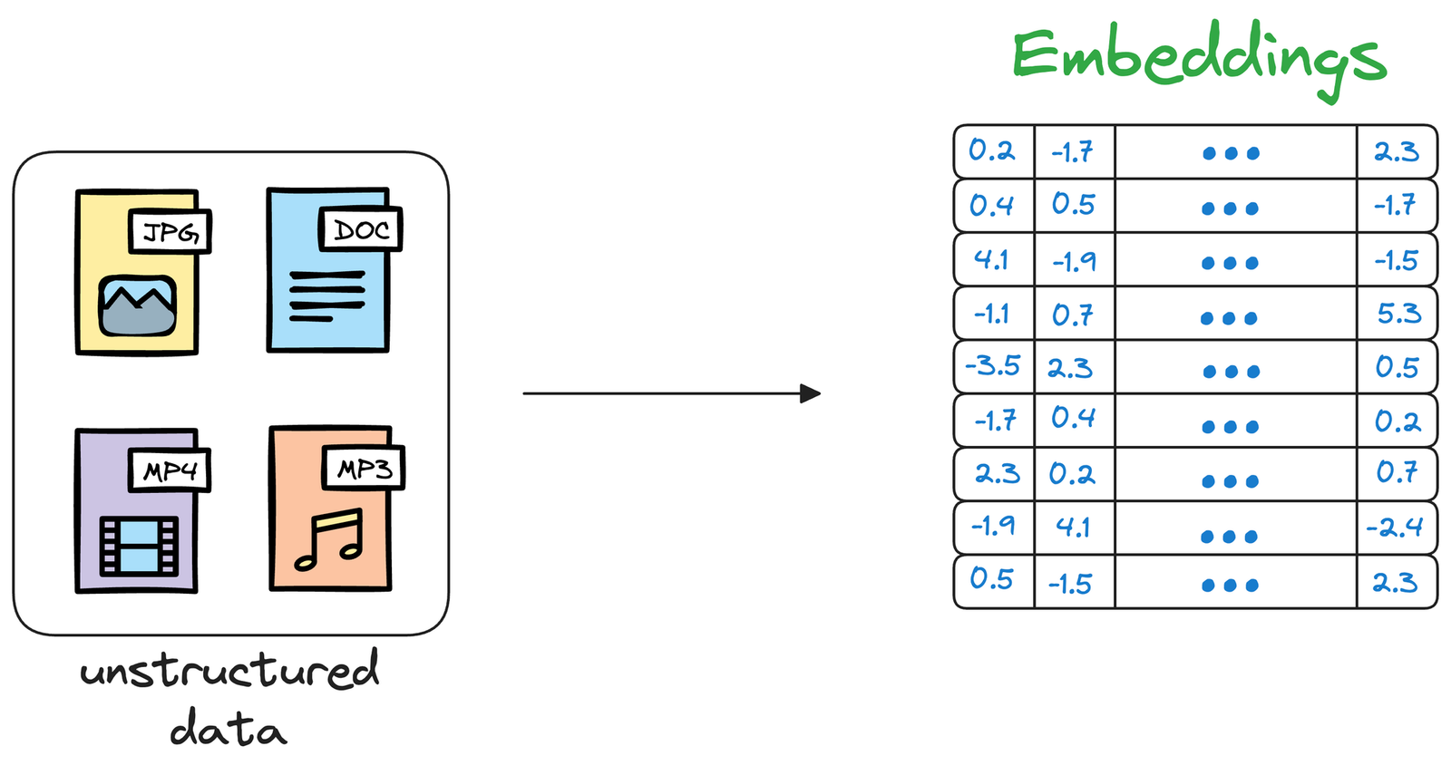
Each row is one embedding — a fixed-length list of numbers standing in for a piece of content. Once everything is numbers, the computer can measure how close two things are.
Those numbers are coordinates on a map of meaning:
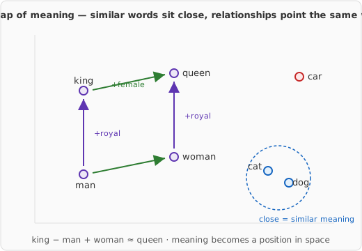
Think of an embedding as a semantic hash. A normal hash function spreads inputs uniformly — two similar strings produce completely unrelated hashes. An embedding is the opposite: it's a hash where proximity in the output space encodes similarity in meaning. That property is what lets the model answer questions about things it's never seen verbatim, and it's the foundation of every semantic search and RAG system you'll build later in the course.
In plain words
Imagine a library where books on similar topics are shelved next to each other — cookbooks
in one aisle, car manuals in another. An embedding is the model's way of giving every word
or sentence a shelf location, so "close on the shelf" means "close in meaning." The famous
party trick — king − man + woman ≈ queen — works because the direction you walk to go
from "man" to "king" is the same direction that takes you from "woman" to "queen."
Embeddings are learned during training — the model figured out these coordinates from billions of examples of words appearing in context, not from a human-labelled dictionary.
The transformer architecture and attention
The transformer is the neural-network architecture behind every major LLM. Its core insight, from the 2017 paper "Attention Is All You Need," is to process all tokens in parallel using a mechanism called attention.
Here is attention without the math: for each token in your input, the model computes a relevance score between that token and every other token — simultaneously. Think of it as every word in a sentence filling out a "how relevant is each other word to me?" ballot at the same time. The model then uses those scores to build a richer representation of each token that incorporates context from the most relevant neighbours.
Inside one transformer layer (stacked N times):
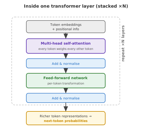
Why does this matter for you as a developer? Attention is why an LLM can track that the pronoun "it" refers to the noun eight sentences ago, resolve an ambiguous "bank" as "riverbank" given the surrounding context, and handle long, complex instructions rather than forgetting them halfway through. The bigger the context window, the more of your prompt participates in this attention calculation — and the more expensive the call becomes (roughly quadratically: double the prompt length and the attention work roughly quadruples, not doubles).
In plain words
Take the sentence "The trophy didn't fit in the suitcase because it was too big." What does "it" mean — the trophy or the suitcase? You know instantly it's the trophy. Attention is how the model figures that out: every word quietly scores how related it is to every other word, so "it" links up with "trophy." Swap "big" for "small" and the answer flips to "suitcase" — and attention flips with it.
Pre-training — what the model learned
Pre-training is the first, enormous training phase. The model is shown hundreds of billions of tokens — web pages, books, code, papers — and trained to predict the next token at each position. That's the entire task: given the tokens so far, what comes next?
From this deceptively simple objective, the model is forced to learn an enormous amount: grammar, facts, reasoning patterns, coding conventions, argument structure, translation, and much more — because producing a good next-token prediction requires implicitly knowing all of those things. The model doesn't memorise facts like a database; it encodes statistical patterns in its parameters / weights.
The analogy: imagine an engineer who spent five years reading every Stack Overflow answer, every technical blog, every RFC, and every open-source codebase, with the sole task of predicting the next word in each document. After that marathon reading, they'd have absorbed an enormous amount about how software works — not by being told facts, but by pattern-matching across millions of examples.
Fine-tuning vs prompting — the key distinction
After pre-training, the foundation model is powerful but not yet useful as an assistant. It has learned to predict text, not to follow instructions. Two fundamentally different approaches bridge this gap:
Fine-tuning is further training — you take the pre-trained model and run another round of gradient descent on a smaller, curated dataset. The weights change. After fine-tuning, the model has literally learned new behaviour at the parameter level. This is what model makers do to create instruction-tuned variants; it is also what you would do (via API or open-weight models) to specialise a model on your company's terminology, tone, or document format. Fine-tuning requires compute, labelled data, and infrastructure.
Prompting changes nothing in the weights. You're sending tokens into a frozen model and relying on patterns the model already knows to steer its output. It's free, instant, and reversible — but constrained to what the model already knows how to do.
The engineer analogy: fine-tuning is sending an employee to a training programme that changes their skills permanently. Prompting is briefing them in the meeting room before a call — useful, but their underlying skills don't change.
RLHF — why models are helpful and safe
A model trained purely on next-token prediction can produce fluent text that is harmful, dishonest, or just annoying to talk to. Predicting what text came next on the internet doesn't teach a model to be helpful — it teaches it to sound like the internet.
RLHF (Reinforcement Learning from Human Feedback) is the training phase that fixes this. Human raters compare two model outputs and indicate which is better — more helpful, more honest, more appropriate. Those preferences are used to train a reward model that scores outputs, and the LLM is then trained to maximise that reward. The result is a model whose default behaviour aligns with "what a helpful human would say" rather than "what the internet says on average."
Every time a modern LLM politely declines to help with something harmful, acknowledges its own uncertainty, or restructures an answer to be clearer — that's RLHF working. It is also why the same base pre-trained weights can produce both a raw completions API and a friendly chat assistant: same weights, different RLHF tuning on top.
Model size — parameters, capability, and cost
Parameters / weights are the learned numbers that define the model's behaviour. A 7B model has seven billion of them; a 70B model has seventy billion; GPT-4 class models are estimated in the hundreds of billions to over a trillion.
More parameters means:
- More capability — larger models handle more complex reasoning, longer context, and edge-case instructions better.
- More cost — every inference call loads those parameters into GPU memory and runs multiplications over all of them. A 70B call costs roughly 10× what a 7B call costs.
- More latency — larger models are slower per token, especially for streaming UIs.
At a glance:
| Model size | Relative cost / latency | Capability | Reach for it when… |
|---|---|---|---|
| Small (~7B) | cheapest, fastest | solid on simple, well-scoped tasks | high-volume classification, extraction, routing |
| Medium (~70B) | ~10× a 7B call, slower | strong general reasoning | most everyday assistant + RAG work |
| Frontier (100s of B–1T+) | most expensive, slowest | best reasoning, hardest edge cases | complex multi-step reasoning, hardest prompts |
For developers, this translates to a routing decision: use a small fast model for high-volume simple tasks (classification, extraction) and a large model only where reasoning quality justifies the cost. Most production systems mix both — a cheap model for the easy 80%, a big model for the hard 20%.
Context window and temperature — the dials you'll turn in Lab 2
Two runtime parameters you'll interact with immediately deserve a brief introduction here:
The context window is the maximum number of tokens (prompt + response combined) the model can consider in one call. Exceed it and the model either refuses or silently truncates the oldest content. Current windows range from a few thousand tokens (small, fast models) to around a million at the frontier (the exact leaders change every few months). The bigger the window, the more context you can include — and the more you pay per call.
In plain words
Picture being on a phone call where your notepad holds exactly one page. You can jot down as much background as fits before the call, but once the page is full, writing anything new means erasing something old. The context window is that one page — and your code, not the model, decides what stays on it.
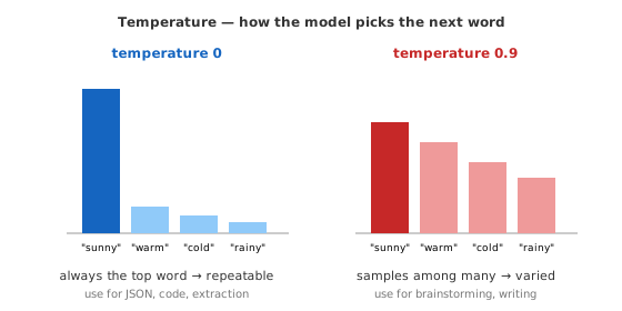
Temperature is the randomness dial: 0 makes the model always pick the most probable next token (deterministic, repeatable — good for structured outputs and tests), and higher values (0.7–1.0) make the model sample from a wider distribution of tokens (more creative, more varied — good for brainstorming and writing). top-p (nucleus sampling) is a complementary control that caps the candidate token pool rather than scaling probabilities; most developers only need to touch temperature.
The same prompt at two temperatures — the model's choice of next word:
KV caching — why generation stays fast
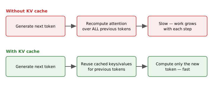
Recall that attention computes keys and values for every token in the sequence. During text generation, the model produces one token at a time: it takes all preceding tokens, runs them through every transformer layer, and predicts the next token. Naively, this means re-running the full attention computation over the entire growing sequence on every single step — work that grows quadratically with sequence length (double the tokens and the work roughly quadruples, not doubles).
The KV cache eliminates this redundancy. After the keys and values for a token are computed in a given layer, they are stored in a cache. On the next generation step, only the newly appended token needs to have its keys/values computed; all prior tokens' cached keys and values are reused directly. This makes generation roughly linear in the number of new tokens rather than quadratic in the total sequence length — which is why you see streaming output appear at a steady pace even for long responses.
The cost is memory: every cached key/value tensor must live in GPU memory for the duration of the generation. This is the primary reason that longer contexts are not just slower to process (the quadratic attention at the prefill stage) but also more expensive to hold in memory throughout generation.
With vs without a KV cache, when generating the next token:
In plain words
It's like writing a long letter. Without a KV cache, you'd re-read the entire letter from the top before adding each new sentence — slower and slower as it grows. With the cache, you just glance at your running notes and write the next sentence. That's why streaming output keeps a steady pace instead of crawling near the end — and why a longer conversation eats more memory (the notes get bigger).
Beyond text — multimodal models
Most models you'll use today are multimodal: they accept more than text — images, audio, sometimes video — and some generate images too. Under the hood it's the same move as embeddings: a picture or an audio clip is turned into vectors the model processes right alongside text. Practically, that means you can hand a model a screenshot, a chart, a photo of a receipt, or a UI mockup and ask questions about it — no separate OCR pipeline required. When you evaluate a model, "multimodal" is now a capability to check for, not an exotic extra.
Reasoning models — paying the model to think first
Everything above describes a model that answers in one fast pass: tokens in, tokens straight out. A newer class — reasoning models (often called "thinking" models) — adds a deliberate step before the visible answer. The model first generates a private chain of reasoning — trying approaches, checking itself, backtracking — and only then writes its reply. Examples: OpenAI's o-series and DeepSeek R1.
The idea has a name: test-time compute — spend more computation at the moment you ask, not only during training. Letting a model think longer on a hard problem can beat simply reaching for a bigger model.
What this means for you as a developer:
- They cost more and respond slower. The thinking is generated as reasoning tokens you pay for, even when you never see them — a reasoning model can burn several times the tokens of a standard call.
- You prompt them differently. "Think step by step" is largely redundant — the model already reasons internally. Give it the goal and the constraints; don't micromanage the steps.
- Use them selectively. For multi-step maths, logic, planning, hard debugging, and tricky analysis, a reasoning model is often worth the cost. For classification, extraction, formatting, and simple Q&A, a fast standard model is cheaper and just as good.
In plain words
A standard model answers instantly, off the top of its head. A reasoning model says "give me a minute," works it out on scratch paper, then tells you the answer — slower and pricier, but far more reliable on genuinely hard questions. The routing rule mirrors model size: default to a fast model; escalate to a reasoning model only when the task truly needs multi-step thinking.
Hands-on
Open Lab 2 — First API Call. You'll make your first direct API call, observe how token counts are reported in the response, and experiment with temperature to see randomness change in real time.
Go deeper
-
Tiktokenizer — Interactive Tokenizer Playground — Paste any text and watch it decompose into colour-coded tokens in real time for GPT-4, Llama, and Claude tokenizers; the fastest way to build token-counting intuition.
-
The Illustrated Word2Vec — Jay Alammar — Diagram-heavy walkthrough of how word embeddings are learned; the clearest visual explanation of why "king − man + woman ≈ queen" works and what embeddings encode.
-
Illustrating RLHF — Hugging Face Blog — The definitive illustrated explainer of the RLHF pipeline: reward model training, PPO, and how human preferences shape LLM behaviour; a short read with clear diagrams.
-
What is RLHF? — AWS — A concise, vendor-neutral reference page covering the full RLHF loop; good for sharing with stakeholders who want a one-page explainer.
Jargon recap
tokenization · token · embedding · transformer · attention · KV cache · pre-training · fine-tuning · RLHF · parameters / weights · context window · temperature · top-p · multimodal model · reasoning model · test-time compute · reasoning tokens
Check yourself
Try to answer before expanding — active recall is what makes it stick.
Why is a token not the same as a word, and why does that matter?
A token is roughly 3–4 characters — a sub-word fragment, so unbelievable can be three tokens. It matters because billing, context limits, and every max_tokens setting count tokens, not words, and non-English text often tokenizes far less efficiently.
What does it mean to say an embedding represents meaning as coordinates?
Each token or piece of text becomes a point in high-dimensional space where similar meanings land geometrically close together. That proximity-encodes-similarity property is what lets the model generalise and is the foundation of semantic search and RAG.
When would you fine-tune a model instead of just prompting it?
Fine-tuning changes the weights via further training, so reach for it to bake in a consistent style, tone, format, or behaviour — when prompting alone can't get there reliably. Prompting changes nothing in the weights; it is free, instant, and your default lever.
When should you escalate from a fast standard model to a reasoning model?
Escalate only when the task genuinely needs multi-step thinking — hard maths, logic, planning, tricky debugging or analysis. Reasoning models burn extra (paid) reasoning tokens and respond slower, so for classification, extraction, formatting, and simple Q&A a fast standard model is cheaper and just as good.
Key takeaways
- Tokens are the model's bytes — billing, context limits, and all runtime math operates on token IDs, not words; one English word is roughly 1.3 tokens on average.
- Embeddings are semantic coordinates: similar meanings cluster together in vector space, which is why LLMs generalise and why semantic search works.
- The transformer's attention mechanism lets every token weigh every other token simultaneously — that's why LLMs handle long-range context so much better than earlier architectures.
- Pre-training bakes in the model's knowledge; fine-tuning changes the weights for specialisation; prompting changes nothing in the weights — just your context.
- RLHF is the difference between a fluent autocomplete and a genuinely helpful assistant; temperature and context window are the main runtime dials you control.